Introduction: What is Information?
At a talk I attended recently, the invited speaker started out by saying that the concept of information was universal, and that nobody could argue about its definition. “Aliens from another planet,” he claimed, “would agree with us instantly about what information is and what it isn't” [i].
…then for the rest of his talk, he avoided giving a clear definition.
I think the problem is that information seems so intuitive (or maybe “pervasive” is the better word) that we don't think a lot about it. However, academics have long arguments about what constitutes information.
In Neal Stephenson's delightful novel “Cryptonomicon”, information is the lead character more than any of the human protagonists. Stephenson weaves a story through several generations, as he writes about the use of cryptography today and during WWII. Sure, Alan Turing's work at breaking the Enigma code was a stunning success for code breaking (and mathematics and computer science in general), but it was only the beginning.
Once US allies broke the Nazi code, they had to make sure that the enemy didn't know they had broken it. If the Germans found out, they would quickly change their encryption method, rendering all future messages unreadable. So, espionage during WWII quickly became a game of not letting the enemy know that you know what they know (ad infinitum). [Stephenson, 1999]
For example, the encoded message is information. But so is the fact that there might be a flurry of cryptographic messages sent right before an imminent enemy attack. Even without breaking the code, information can be “extracted” of a sort. Knowing where the message was broadcast from (and more importantly perhaps, where it is being sent to) is a third form of information, perhaps called “metainformation”. Or, knowing the form the message was sent in: radio, written, or telegraph, is another bit of information. The coding scheme, and the fact that the message was encrypted at all is a piece of information.
Two Opposing Views
As Marshall McLuhan noted, “the medium is the message” [ii]. McLuhan is often misinterpreted here as talking about information theory. Instead, he was making a point about the personal and social consequences caused by any new technology. He gives electric light as an example of pure information, since whether it is used for “brain surgery or night baseball”, it has given birth to brand new activities that were impossible before it was invented. The fact that the light has no information content by itself is irrelevant [McLuhan, 1996 (original essay,1964)].
Meanwhile, in the book Feynman and Computation (which include Feynman's seminal essay “Plenty of Room at the Bottom”), Rolf Landauer argues that information is inevitably physical. [Landauer (Hey), 1999] There must be a tangible representation, or else it can't be stored. Feynman himself envisioned the entire Caltech library of 120,000 volumes stored on a single index card [Feynman,1959]. However, with Claude Shannon's connection of information and entropy, it can be shown that information will tend to disappear and decay over time. Early computer pioneers worked hard to increase the amount of time (called big “T”) where information could be stored in delay lines, long before dynamic memory was invented.
For the purposes of this paper, we can assume that information is stored in a linear, ordered set of numbers. To make things easier, we can restrict the sequence to binary 0 or 1 values, since any number, decimal, octal, or hexadecimal, can be represented as a binary value. This idea was first published by Swiss mathematician Jakob Bernoulli in 1713 in his “Ars Conjectandi” (Beltrami, p. 5). The series of ones and zeros forms a binomial distribution that can be analyzed by a binomial random variable, usually defined as the number of ones represented in the string of n digits. (Of course, you could count the number of zeros, too, but you'd get the same results mathematically).
Characteristics of Binary Messages
For the definition above, the information content says the same, regardless of how it the message is transmitted, how long transmission takes (or when the message starts and stops), or any other “meta-information” about the message. This is actually a very difficult condition to meet, for the reasons stated above. In reality, we often find out more information content from those auxiliary characteristics than from the message itself.
In his famous 1948 paper, “A Mathematical Theory of Communication”, Claude Shannon notes that the “semantic aspects of communication are irrelevant to the engineering aspects”. [Shannon, p. 31]. That is, we can ignore the other aspects of information, and concentrate on the mathematical characteristics of the binary signal. In that paper, Shannon described the first useful metric to measure the information content in a binary message. This measure of information “entropy” is still used today. You can note that the original title to Shannon's paper has now turned into “The Mathematical Theory of Communication” in later editions.
In Shannon's scheme, a unit of information has an entropy measure proportional to its probability times the log (base 2) of the probability. In his example, imagine we have a message made up of the letters A, B, C, and D, with the respective probabilities of: 1/2, 1/4, 1/8, and 1/8. [Shannon, p. 63] So the total entropy for the message is the sum of the p logp of each element:
![]() bits per symbol
bits per symbol
The logarithmic function has the attractive property that it is additive, and appears often in engineering problems (Shannon, p. 32). It also has the nice property that the curve of the entropy function p logp is bounded by 0 and 1 for any probability. For example, if we take the probability q to be (1-p), the function h = 1(p logp + q logq) looks like this:
Figure 1: H = p logp + q logq
So, H itself can be used as a probability function! Even better, the graph above shows us that the maximum entropy will occur when the probabilities of p and q are equal. That is, when p = 0.5, then (1-p) also equals 0.5, and the distributions are equally “mixed”. Likewise, for three variables p, q, and r, the maximum cumulative entropy will occur when they all have a probability of 1/3. In general for n probabilities, they will all have probability of 1/n.
Some researchers have dubbed this a measure of the “novelty” of the signal. Novelty detection in an important topic in artificial intelligence, because autonomous agents need to separate new and important data from the constant stream of random information they receive every second from the outside world. There are papers that use hundreds of different methods to perform the task: clustering, self-organizing maps, linear programming, and neural networks. The topic has many applications in other fields, too, including signal and speech processing, psychology, cognitive science, and biology.
However, most of the results so far from researchers show that the representation of the data is extremely important. If you can transform the data into a “good” set of inputs, often the classification task is easy. However, how to perform that transformation of every possible set of data has not been solved yet.
Coding Theory
In out previous examples, the data has been written down as ones and zeros, without thinking about what those digits mean. However, in most cases, the numbers represent an underlying message that we are trying to convey: “101” could be translated into the number “5”, or perhaps it symbolizes two state transitions — one from 1 to 0, and the next from 0 to 1. Shannon gives an example of a message of three letters A, B, C, and D, encoded as the following:
A = 00                  C = 10

B = 01                  D = 11
The total average length for the message = N(1/2 x 2 + 1/4 x 2 + 2/8 x 2) = 2N. However there are better possible encoding schemes. For example, if we try:
A = 0                   C = 110

B = 10                  D = 111
Now, the total average length is N(1/2 x 1 + 1/4 x 2 + 2/8 x 3) = 7/4 N. This the a better encoding scheme, since 7/4 < 2. This is also the best possible encoding scheme possible, according to Shannon. In fact, there is an absolute bound on how much any data stream can be compressed without loss of information. This is the reason that computer modems can't transmit any faster than 56 kilobaud per second over standard US telephone lines. There is a whole industry built around trying to find better encoding schemes, and there exist algorithms that adapt in “real-time” to the incoming data.
To find the best possible lossless coding scheme, we can use a “Huffman Code”, invented by David Huffman in 1952. The method is known as a “greedy” algorithm because it always takes the best local choice at any moment in time. Other algorithms need to balance local choices with negative global effects that might occur at a later stage, but Huffman works by taking the best choice it can easily see in “one step”. Here is some pseudo-code that operates on a list of n units that make up a message C with a given set of frequencies: (from CLR, p. 340)
Huffman(C)

n
← |C|

Q
← C

for
i ← 1 to n −1

     do
x ← Allocate-Node()

     x
← left[z] ← Extract-Min(Q)

     y
← right ← Extract-Min(Q)

     f[z]
← f[x] + f[y]

     Insert(Q,z)

Return
Extract-Min(Q)
It's not readily apparent from the precious code, but what the algorithm is doing is finding the two units with the smallest frequency and combining them into a new unit with frequency f[z] = f[x] + f[y]. This forms a binary tree-like structure with nodes that have left and right children. Of course, a unit might be combined more than once, and the tree can have a very complex structure.
To return to our example, we have n = 4 units. We can place these initially in any starting order:
![]()
The two lowest frequencies are C = D = 1/8. So, these would be combined to form a new unit with frequency 1/8 + 1/8 = 1/4.
Continue the process and merge the two units with the next-lowest frequencies. For our example, the new unit “New CD” and “B” both have frequencies of 1/4, so we combine these into a new unit of frequency 1/2.
To find the final coding scheme, start at the top node, and trace a path downward to each final “leaf” node. Moving to the left will represent a “0” and moving to the right will be “1”. Note that by doing this, we a performing a “depth-first” search of the binary tree. In any case, the first node “A” corresponds to the code “0”, while “B” will be represented by “10”, and so on.
This will turn out to be Shannon's suggested coding scheme, and you can prove that it is optimum (see proof of Huffman's algorithm on p. 342 of CLR). In fact, the average length of the encoding will approach an absolute bound that equals the entropy function H!
All Information Is Not Created Equal
All of Shannon's formulas above assume a discrete noiseless system. If our channel is dropping bits or corrupting the information, of course the entropy will go up and the message will slowly be lost. Shannon anticipated this with an associated theory of discrete channels with noise. For example, if we need to transmit each bit twice, the entropy and the average length of transmission both double.
There are better methods we can use to verify that information has been received correct. The simplest of these is a binary “single-parity-check” (SPC), which adds up the bits in the preceding signal. If the result is even, “0” is used as the parity bit. If the result is odd, “1” will be transmitted. However, with this scheme, two things have happened. First, because the parity bit doesn't convey any information by itself, it could be lost without destroying any information. However, it isn't treated the same as all the other bits so evidently, “All information is not created equal”. Second, adding parity bits increases the length of the message, so we have changed the overall entropy of the message in a complex way.
The number of digits between parity bits need to be determined by the error rate. If “1-to-0” errors are more prevalent than “0-to-1” noise, the length needs to be a function of the message itself. But at the same time, the length of the “frame” needs to be set even before any information has been transmitted, or decoding the parity bits will be impossible. So, there are adaptive schemes where the number of parity bits and their frame sequences changes over time, depending on how well the communication is occurring.
The Pioneer 10/11 Plaque
If we were sent a message from an alien intelligence, what would it look like? Well, to our knowledge, we have yet to receive one. However, we have sent many messages to outer space, so we might as well ask what those messages look like.
On March 2, 1972 we launched the Pioneer 10 spacecraft and a year later on March 6, we launched Pioneer 11. Both spacecraft were designed to travel outside out our solar systems, and both carried a 6-by-9 inch gold-anodized metal plate that represented our message to any alien civilizations that might stumble upon it. The plate was engraved with a picture representing several icons that a team of NASA researchers (including Carl Sagan) spent three weeks to design. [iii]
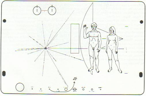
Figure 2: Plaque from Pioneer 10 and 11
First, without looking below, try to guess what the symbols are supposed to represent.
The circle in the upper-left corner forms a representation of the “hyperfine transition” of a neutral hydrogen atom. The lines above each “binary 1” reflect the transition from antiparallel to parallel spins of the nucleus and electron, but as Sagan notes, “so far the message does not say whether this is a unit of length (21 cm) or of time (1420 MHz)” [Goldsmith, p. 275]. The NASA team added three small dashes to the right of the female figure, which equate to a binary value of 8, but it doesn't really clear up what the units are. So, the aliens that find this plaque are supposed to figure out that the value of 8-by-21 is supposed to correspond to the dimensions of the Pioneer spacecraft drawn behind the woman. I am not an alien, but I would be confused about the 8-by-21 reference. The key if to multiply 8 by 21 centimeters to get the proper height of the human woman, and not to think of 8-by-21 as being height and width measurements.
The planets at the bottom of the plaque seem familiar enough, even if they are not to scale. Worse, they are all in the same line, and not in the usual solar orbits. There is a dashed code here, too, but this time, the aliens are supposed to know which the addition of a tiny “serif”, that the units are different than the ones used previously, and that they are all scaled as multiples of the distance from Mercury to the Sun. Sagan again apologizes, “There is no way for this unit of length to be deciphered in the message”… but hopefully the aliens will realize that half the plaque refers to exact distances, while the other half represents a relative scale.
The lines bursting out of the left side of the plaque are interesting. They are a “map” of sorts of the sun with respect to fourteen pulsars and the center of the galaxy. The lines are actually binary digits again, but this time they are supposed to represent time intervals, and not distances. The fact that there are ten decimals digits should lead the aliens to realize that human beings couldn't measure distances to ten digits, and even if we could, those distances change rapidly as the universe expands. So, if the high precision represents time, then only pulsars would have a property that could be measured precisely. Well, almost precisely. For two of the pulsars, we only have seven digits of precision, and a broken line and several zeros are supposed to tell the aliens that we're not quite sure about those periods yet.
Ok, even if we grant that we have the relative distances between fourteen pulsars, they are drawn in a flat plane. Even though we weren't sure in 1972 of the distance from the earth to many of these pulsars, a radius “r” is given next in binary notion. Then, there is an angle θ and a polar coordinate z. There is no reference to which direction is “up” or “down”, polar north or south. There was supposed to be a + or − sign denoted by the spacing of the tick marks leading to each pulsar, but the engraver who made the plaque made a mistake. The long line leading to the right behind the human figures give the distance to the center of the galaxy, hopefully giving the aliens proper directions on how to visit us.
The less said about the male and female figures standing on the right side of the plaque, the better. Carl Sagan notes how the figures were supposed to be racially indeterminate, and how they wanted to show off our ten fingers, ten toes, and our opposable thumbs. Electronic musician Laurie Anderson quips, “In our country we send pictures of people speaking our sign language into outer space. We are speaking our sign language in these pictures. Do you think that they will think his arm is permanently attached in this position? Or, do you think that they will read our signs? In our country goodbye looks just like hello. Say hello. Say hello. Say hello.” [iv]
The Voyager Records
In my opinion, the Pioneer 10/11 plaques were a mistake. There are seven different units of measurement, and no two alike. One represents time, one absolute distance, two that are multiples of the absolute distance, and a confusing (r, θ, z) notation that was screwed up by the engravers. Even if the aliens manage to break our code, they still have a complex problem to solve, when they try to find fourteen pulsars in the galaxy with the given properties… hoping that there relative distances and periods haven changed very much. I don't think Pioneer 10 and 11 could find their way home with such a bad map.
Of course, part of the problem is that the NASA team was given a small two-dimensional area to convey some complication information. Sagan talks about some ideas that were discussed that didn't make it onto the plaque: radioactive time markers (rejected because they would interfere with the Pioneer radiation detectors), representations of biological systems such as our brain, or a stellar map (rejected because of problems of representing stellar motion). Surely there is a better medium to communicate this complicated information.
The later Voyager 1 and 2 spacecraft both carried a copy of a 12-inch copper record, designed to be played at 16 2/3 revolutions per minute using a ceramic stylus included on the spacecraft. There are instructions on the lid of the disk's container describing how to decode the record, but of course they are pictograms and not written in any language. Assuming, the aliens can figure out how to construct a turntable, they will be able to hear sounds as well as “see” 116 pictures. Decoding the pictures might be tricky, since there aren't any instructions on how to translate it into a matrix or color bit structure, but if it works, the aliens will be able to see:
- A calibration circle that defines scale and dimensions for the rest of the pictures
- A crocodile
- Heron Island in Australia
- Chinese Dinner
- “Old Man with Dog and Flowers”
- Supermarket
- India Rush-Hour Traffic
- “Licking, Eating, Drinking”
- Cathy Rigby
- “Cooking Fish”
…among other pictures. Even though there are other photos of human development and conception, it's a rather odd selection. There's the word “hello” in sixty languages, including Amoy, Gujarati, Hittite, Kannada, Kechua, Luganda, Nguni, Nyanja, Oriya, Sotho, and Telugu. Even considering that the disk was created in the awakening social liberalism of the seventies, it's still an impressive list. Then, there are several audio sound, including:
- Mud Pots
- Herding Sheep
- “Kiss”
- Cricket Frogs
- Riveter
To finish off this eclectic CD is a programme of light music, including Bach's “Brandenburg Concerto #2”, Mozart, Louis Armstrong singing “Melancholy Blues”, Navajo chants, and Chuck Berry's “Johnny Be Goode” (!). I guess we should be happy that the Voyager spaceships were launched before the invention of rap music.
Electromagnetic Signals
Music seems to be a step in the “right” direction, if only because linear signals can convey many different things. For example, the signal from the Voyager record was able to represent both pictures and sound, as well as the idea of scale and intensity. Plus, electromagnetic energy travels at the speed of light, while the Voyager 2, traveling at style='font-family:Arial;color:#000033'>56,000 kilometers (35,000 miles) per hour, will need thousands more years to reach the vicinity of the next nearby stars. Space is an extremely big place, and the chance of finding a powerless spacecraft is quite small.
Broadcasting in the electromagnetic spectrum, however, is not without its drawbacks. The largest problem is that the spectrum is filled to capacity with terrestrially produced signals that clutter up the airwaves. style='font-family: Arial'> The first signals that human beings sent into outer space was in the 1870s, when Heinrich Heine tested James Clerk Maxwell's theories on the propagation of electromagnetic waves. Thirty years later, Gugliemo Marconi created the modern radio, which became quickly adopted. Today, the frequencies from 9 to kHz, with AM radio from 535 to 1605 kHz and FM from 88.0 to 108.0 MHz. Meanwhile, television signals are intermittently from 470 to 806 MHz, with a gap from 608.0 to 614.0 MHz reserved for radio astronomy. Other bands are reserved for maritime and aeronautical signals, amateur (ham) radio, cellar telephones, and a thousand other special-use allocations and permits from the FCC. [v]
The 1974 Arecibo Message
In 1974, the Arecibo Observatory sent a message into outer space, designed as the first attempt to contact another civilization with a coherent message. They increased the power of their transmitter to an unprecedented 2x10¹³ Watts of power, some 20 times the generating capacity of all the electrical power stations operating at the time, all combined! [vi]
They chose a frequency of 2380 MHz, where there is a convenient gap in the allocated spectrum reserved for radiolocation, and a bandwidth of about 10 Hz. With that small bandwidth and power, they predict the message could be detected throughout the galaxy by any radio telescope comparable to the one at Arecibo. The effective radiated power in the direction of the transmission was 3 x 10¹² Watts, the largest signal ever radiated before (or probably since). The transmission was directed at a globular cluster of stars (the Great Cluster in Hercules/ Messier 13), which comprises about 300,000 stars in a small area. However, since that cluster is about 25,000 light years distant, it will be a while before we know if our message is received.
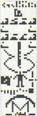
Figure 3: The 1974 Arecibo Message
Again, it's kind of fun to try and figure out what the message means before reading on:
The transmission starts with a “lesson” on the binary notation used in the message. Written from right to left are the numbers from 1 to 10 written in that notation. The most significant bit is at the top, and at the bottom is a “number label”, marking where each number is located.
Next is a series of numbers: 1, 6, 7, 8, and 15. This sequence is supposed to represent the atomic numbers of hydrogen, carbon, nitrogen, oxygen, and phosphorous. This allows the next cluster of bits to represent the physical structure of several interesting molecules, such as sugar (deoxyribose), and the components of DNA: thymine, adenine, guanine, and cytosine.
Next, as you can expect, is a representation of the double-helix structure of DNA. Inside the graphic representation of the coiled helix is a number (note the number label specifying where it starts and stops), suggesting that there are over 4 billion pairs of the elements above which comprise our DNA. So, even if this message doesn't have the instructions on how to build a spacecraft (unlike the message in Carl Sagan's book “Contact”), we have at least given aliens some instructions on how to build a human being. Perhaps they would try to build their own example!
The structure of a human being is placed below the DNA, along with a “ruler” suggesting that the person is 14 units high. The “unit” in question is the wavelength of the Arecibo transmission itself, about 12.6 centimeters. This makes the average human being about 5′ 9.5″ tall. On the other side of the figure is the number 4 billion, which is meant to represent the population of Earth (which thirty years later is off by about 2 billion).
Finally, there is a graphical representation of the solar system (with Earth “highlighted”) and a picture of the Arecibo telescope. It is pointing downward to suggest that the message is being beamed from the highlighted Earth. The last bits of the message represent the size of the Arecibo dish. It is 2430 wavelengths across, or about 1004 feet wide.
So, the Arecibo transmission is a bit clearer on the scale and format of the binary notation used in the message. It is missing a “map” similar to the Pioneer plaque, but it contains a lot of other interesting information. One minute after its transmission, it had already traveled as far as the distance from the Sun to Mars. After 71 minutes, it had passed Saturn, and a little later, both the Pioneer spacecraft, leaving the idea of physical data far behind.
What is Randomness?
Human beings are terrible at recognizing randomness. In one test [vii], subjects were asked to choose which of the following sequences was random and which the researchers invented:
0 0 1 1 0 0 0 1 0 1
0 0 0 0 0 1 0 1 0 1 1 0 0 1 0 0 1 0
or
0 0 1 0 1 1 0 1 0 1
1 1 0 0 1 0 1 0 0 1 1 0 1 0 1 1 0 0
Most subjects said that the second sequence seemed to be a lot more random. The five zeros in a row in the first sequence looked suspect, as well the fact that there are only 10 out of 28 ones in the first sequence, compared to the 14 out of 28 they expected to find that are shown in the second sequence. This is confusing, because human beings are normally inclined to see patterns where none exist. For example, the fact that people can see faces (or pictures of Jesus Christ) in puddles and tree trunks hints that the brain is hard-wired to recognize faces. [viii]. Or, as John Cohen says, “What they appear to tell us is that nothing is so alien to the human mind as the idea of randomness.”
In actuality, the first number is the first seven digits of π: 3141592, written in four-digit binary numbers. For the second number, I studiously made sure that the numbers of ones and zeros matched, and that there weren't any strings of five digits in a row that were the same.
Actually, for a 28 digit number, the probability that there is a sequence of four (or more!) zeros or ones in a row is about 100%. Think of it this way: there are sixteen possible sequences of four ones and zeros (shown below in Figure 4). The chance that a “1111” will appear given any four digits is 1/16. Doing this seven times gives a probability of 7/16 that a “natural” 1111 will appear. Of course, other combinations of 1111 can be made, such as a seven followed by an eight or nine (0111 + 1000 or + 1001), pumping the probability over 50%.
Similar reasoning can be made for four (or more) zeros in a row. So, the chances that the second sequence could appear randomly (with the longest running sequence being three measly ones in a row), is quite small.
    0000 = 0            0101
    = 5
    0001 = 1            0110
    = 6
    0010 = 2            0111
    = 7
    0011 = 3            1000
    = 8
    0100 = 4            1001
    = 9
Figure 4: Table of binary digits for pi translation
As far as randomness goes, the first sequence using pi is more random. Even if we discover the “meaning” or creator of some series, it doesn't make the numbers any less random. There is some bias since there are no numbers “greater” than 1001 = 9 that can be used in the sequence… so no “1111” would appear naturally. However, as noted above, sequences of four ones can appear in other ways. This is often called a “run test”, testing the probability of the existence (or absence) or the longest continuous string of digits.
Similar to the “run” test is the “gap” test, which measure how many “non-zero” (or “non-one” digits are between any two zeros or ones. For binary sequences, run and gap tests are the same thing. However, if we were dealing with decimal numbers, gap tests might be more useful that run tests, where the possibility of five “eights” in a row might be so small that it is dwarfed by the sample size n. Both of these tests are known as “serial”, because the order of the digits is extremely important. In this fashion, they are more like the number sequences discussed later than tests on random numbers themselves.
Testing the 1974 Arecibo Message
All of these tests are simple hypothesis tests. A sequence of binary numbers is a binomial distribution, much like flipping a coin. We can count up the total number of zeros or ones in the sequence to make sure that it equals 50% (i.e. an unbiased probability).
A binomial random value can be approximated by a normal distribution if np > 10 and n(p-1) > 10. For the 1974 Arecibo message mentioned before, n = 1679 and p is expected to equal q, and both should be 0.5. So, np = (1679)*(0.5) = 839.5 which is a lot larger than 10. So, we can go ahead and look at a normal distribution. However, looking at the actual ones and zeros of the message gives the totals below:
Number of ones
expected = n/2 = 1679/2 = 839.5

Number of ones actually
in message = 397

P(1) = 397/1679
≈ 0.23645

Likewise, P(0)
≈ 0.76355
Are these results out of line? Do they prove that the Arecibo sequence is not random? Well, we need to perform a hypothesis test where the hypothesis “Ho” is the idea that the P(1) = 0.5. The “alternate hypothesis Ha” is the idea that the probability P(1) < 0.5.
For our data, the test statistic value z is:
 =
=
We want to reject Ho in favor of the alternate hypothesis if the value of z is less than a chosen z. For example, at a “significance level” of 0.01 (or in other words 1% confidence that we are correct), z0.1 is −2.33. Since z is really small:
Z = -0.23645/0.012202387 = -21.59824 which is much smaller than −2.33
In fact, we could use an extremely small significance level of 0.001 (or 0.1%), and still be reasonably sure that the fact that there are so few zeros hints at the idea that the 1974 Arecibo message is random.
Conditional Probability
We could imagine strings where P(0) ≈ P(1) ≈ 0.5, but the message is still probably not random. For example, the following string definitely has a pattern:
0 1 0 1 0 1 0 1 0 1
0 1 0 1 0 1 0 1 0 1 0 1 0 1 0 1 0 1 0 1
So, we can test the conditional probability of each of the numbers. For example, the probability of a one following another one should be the same as a zero following that one. Statisticians would say P(0|1) needs to be equal to P(1|1). This is similar to combining the Arecibo message in groups of two, and making sure that there is the same number of “00”s as there are “01”s, “10”s, and “11”s. They should all have a probability of 0.25.
This is known as a “serial test”, compared to the earlier “frequency test”. We could do the same thing with groups of three, then four, and so on. However, on second thought, doing groups of four is the same things as examining groups of two. For example, if the all four digits sequences “0000” through “1111” come up with equal probability, we don't need to look at “00”, “01”, “10” and “11”. In that case, all even numbers less than six have been “covered”. One scheme would be to look at all prime sequences of numbers; make sure that we examine groups of 1, then 2, then 3, 5, 7, 11, and so on.
Approximate Entropy
However, where should we stop? Our Arecibo message is only 1679 digits long. If we look at sequences of 1679 digits, there will only be one of them represented in our data. Clearly, we have hit upon the limitation of our “small” sample size. Our tests only work if np > 10. If each group we are testing has leangth m, there are 2m possible combinations of the digits 0 and 1. Since we expect to have an equal probability for each of our groups of numbers, we want p = 1/2m. Similarly, the number of possible groups n depends on the length, too, as n = 1679/m. So, we solve (1679/m)( 1/2m) > 10 to know that the largest m we can test is sets of only 5 digits. Clearly, this doesn't give us many hypothesis tests that we can perform, since m = 4 is so similar to m = 2.
In 1997, Steve Pincus suggested the use of “approximate entropy” as a measure of the randomness of a number. Pincus, a freelance mathematician from Guilford, Connecticut, (as well as Burton Singer of Princeton University and Rudolf E. Kalman of the Swiss Federal Institute of Technology, Zürich), used the ideas of Kolmogorov and Solomonoff to develop a new definition of complexity. In this definition, the number must equal numbers of ones and zeros, as well as pairs, triplets, and so on, up to sequences of length log2 log2 n + 1. [ix]
So, for the thirty-two possible five-bit sequences 00000 through 11111, only 00110, 01100, 11001, and 10011 are pronounced as random. The digits of pi also passed the test as random. Note that if we look at sets of two numbers, there are only four possible choices: 00, 01, 10, and 11. Each of these has a probability based on its presence in the input string. So, we are back to the original definition of entropy:
![]()
If we perform this test on bigrams (groups of two digits) and then move to trigrams (groups of three), how much information about the randomness of the signal have we added? This is the “ApEn(k)”, or approximate entropy of the difference between block of length k and those of length (k-1):
![]()
Using some approximate entropy code written in MATLAB [Beltrami, p.165], I tested the 1974 Arecibo message against four other signals: all ones, a normalized sine wave, alternating zeros and ones, and a completely random signal using MATLAB's built-in random number generator. However, I couldn't get the sample code included with Edward Beltrami's book to work for a grouping constant “k” higher than 1. There were several typos, and I wasn't exactly sure how Beltrami was using a hard-coded permutation matrix. However, I reach some interesting results:
All
ones:               -8.9658

0
1 0 1 0 1 0 1…:       1

1974
Arecibo Message:   6.6308

Sine
wave:              8.9542

Random
Signal:          8.9658
I think it is interesting that a signal of all ones is the lowest score, while a random signal is the highest score. Even better, they are equal but with opposite signs. It would have been interesting if I had normalized the results from 0 to 1. The ordered signal [0 1 0 1 0 1…] was a value of 1, just about the midpoint of the two values. The 1974 Arecibo Message was a lot more random, but not quite as random as the completely random signal. I think the reason a sine wave was reported as more random than the Arecibo signal was because I used a grouping of k = 1. I'm sure if I used higher values of k, I would eventually surpass the periodicity of the sine wave and it's value would go dramatically down.
Spectral Tests
“Spectral tests” are used to measure regularity in a signal. For example, a sine wave has an extremely regular period (defined as its frequency), while pure noise doesn't have any repeating cycles at all. One way to test regularity is to “correlate” the signal with itself.
A correlation function measures the similarity between two functions x and y by multiplying the first term of x with the last term of y. Then, the next term of the correlation function is calculated by multiplying the first term of x by the “next-to-last” term of y, and adding that to the second term of x multiplied by the last term of y. Performing an autocorrelation is simply equivalent to calculating the function using the same signal twice:
![]()
A better way of thinking about this is to take the signal and copy it. Then, “flip” the signal backwards, and slide it along the original signal, multiplying matching term and adding the resulting series together.
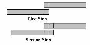
Figure 5: Autocorrelation example
As an example, here is a sine wave autocorrelated with itself.
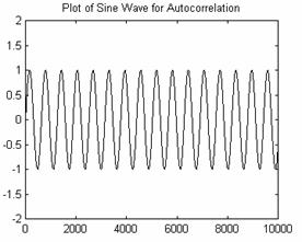
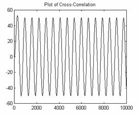
Figures 6 and 7: Sine Wave and Autocorrelation
Meanwhile, examining the 1974 Arecibo Message shows very little regularity:
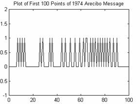
Figure 8: Arecibo Data
Figure 9: Autocorrelation of Arecibo data
Performing a correlation is similar to multiplying the Fourier transforms of the two signals together point-by-point. So, we might as well look at the FFT directly. Since there are 1679 units in the message, we get a Fourier transform of 1679/2 = 839 points. The result looks a lot like the previous autocorrelation, as it should:
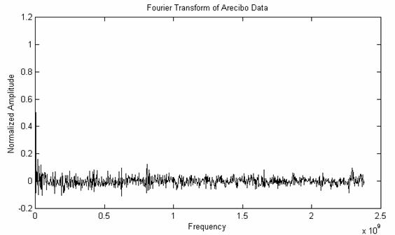
Figure 10: FFT of Arecibo Data
Again, this graph doesn't show any outstanding patterns of regularity. We don't even see anything strong corresponding to the 23-by-73 matrix of the message itself. For example, if there was a single “1” repeated for every 23rd element, regardless of any other data bits, we would expect a peak at the corresponding frequency:
(23/1679) * 2.380 x 109 = 0.0336 x 10⁹
Or, for the 73rd element, we would get a peak at (73/1679) * 2.380 x 109 = 0.103 x 10⁹. However, just looking at the graph above, those peaks are small. Performing more statistical analysis shows that they are there, but they are overshadowing by the rest of the signal. For example, since we showed earlier that there are more zeros than ones in the signal, this will be reflected as a “bias”, and will manifest itself as a huge peak at f = 0 MHz.
I think the Arecibo signal would have been more successful if it would have had a distinct “frame” that was placed every 23 bits. This would make the FFT easier to detect compared to random noise, and would perhaps provide a hint about the 23-by-73 regularity and which way the matrix should be oriented.
Other Randomization Tests
Another randomization test is called a “poker” (or partition) test, where the series is divided into five-digit block, and the results are compared against the expected occurrence of certain five-card poker hand [Bennett, p. 171]. There are also “chi-square” statistical tests, the “Kolmogorov-Smirnov” test, the “coupon collector's” test, permutation tests, and examinations on subsequences of the original data. [Knuth, pp. 34-66]
Which one of these randomization tests is best? What happens if two tests contradict each other; one says the number is random, while the other say it is not? Worse, there is no clear definition is we have succeeded in finding a random number. We have only managed to prove or disprove a given hypothesis that tests for a single characteristic of the data, be it a run sequence or a balanced number of ones and zeros. Of course, when generating a 100-digit number, there is a small (but finite) probability that the sequence will be made entirely of ones.
Here's another question: can we have periods of non-randomness in an otherwise random number? What determines where those patches start and stop? As Peter Bernstein comments in his book “Against the Gods”, the situation is similar to a court of law where the criminal defendants do not attempt to prove their innocence, but rather, their lack of guilt [x]. Or, Keane points out that we can have relative randomness in the same way that we can have relative accuracy without having knowledge of absolute accurate measurement [xi]. For example, we could measure a sheet of paper to be 8.5 inches long. With a better ruler, we could find the width to be 8.501, then 8.50.163, and so on. When do we stop? Perhaps we can never have the exact measurement, but we can possibly define when we are “close enough”. In a similar way, we could say when a number or sequence is “random enough”. Choosing the winner of a bake sale might be more casual than picking the Powerball lottery.
Random numbers
John von Neumann once stated that it is “easier to test random number than it is to manufacture them.” [xii] So, if we were in charge of the lottery, what is the best way to pick the winning combination?
In the 1920s, Leonard H.C. Tippett came up with a list of 5,000 random numbers by mixing up small numbered cards from a bag. However, this method proved to be time-consuming and hard to do. So, he tried again, and came up with a list of 40,000 digits taken at random from a table of local census data. In 1927, Cambridge University Press actually published an entire book made up of Tippett's random numbers — definitely boring reading, but an essential tool for statisticians of the time.
In fact, the book became so popular that other books came out soon afterward: a list of 15,000 numbers selected from the 15th through 19th decimal places of a logarithm table, and 100,000 numbers produced by a machine that used a spinning circular disk. However, all of these methods reflected a little of the methods that were used to produce them. For example, Tippett's census data might have more even numbers in it, since more couples live together in houses that single people.
So, in 1949, the Interstate Commerce commission published a new report with 105,000 random digits that were compiled from mixing all the other previous tables. For example, you could take ever third random number from Tippett's table, or perhaps write down every fourth term backwards. Or, you could add several random numbers together and take the last several significant digits, since any linear combination of random numbers will be random also. However, the need for good random number tables increased until 1955, when the RAND corporation published a book of one million (!) digits.
With the invention of modern computers, we were able to get as many random numbers as we could ever want. In 1951, John von Neumann published a simple algorithm to generate random numbers: Pick an initial number of length n, square it, take the middle n digits of the result, and repeat the process. However, this method is flawed for many initial values. For example, taking the number 3,792 and squaring it gives 14,379,264. Throwing away the first and last couple of digits leaves us with the same number we started with! [Bennett, p. 142]
So, modern random number generation usually follows one of three methods: a generator based on number theory, “congruential” generators that use the remainders of division operations (or modular arithmetic), or generators based on the bit structure of computer-stored information. A new method called “add-with-carry” and “subtract-with-borrow” generators use the Fibonacci sequence (defined later in the paper). Personal computers today sometimes have hardware-specific random number generators, or they use other physical properties of the computer that are random, such as small changes in the clock speed or a heat sensor. Or, some programs use human interaction to form the “seed” that forms the starting conditions of the random number generator. For example, the number of second it takes to get the hard disk “up to speed”, or a time interval between the last two keyboard clicks can be used to form a random number.
One anecdotal story talked about a casino that wasn't very careful with the random number generator in its slot machines. One lucky gambler figured out that if he cycles the power to a machine, it would always start up in the same sequence. After two plays, he would get a large win. Repeating the sequence led to a huge loss for the casino. [xiii]
Random-Like Codes
So, if we have a hard time saying that a signal displaying regularity is man-made, can we say the opposite: a random signal has no information? Again, this is impossible to do. For example, we could take a signal that displays non-random characteristics (as defined by one of the tests described earlier), and insert extra bits into the message in a pre-determined pattern. By analyzing the original message, we could balance the extra bits so the resulting signal passes the randomization tests it previously failed.
One method is called “soft-output” decoding, where the probability of the input is modified by extra information, such as adding Gaussian noise to the signal. One example is a two-dimensional single-parity-check bit. Imagine that we have a number with a parity check bit at the end:
  0


  1


  0


  1


  0
Now, imagine that we add a second four-bit string a calculate the parity bits not only horizontally, but vertically as well:
  0


  1


  0


  1


  0


  1


  1


  0


  1


  1


  1


  0


  0


  0


  1
Final string = 0 1 0 1 0 1 1 0 1 1 1 0 0 0 1
It would seem as if we have added a lot of extra bits into the message, but actually, the ratio of SPC codes to actual data is fixed proportional to the length of the input data. As the data grows by n x m, the length of the parity check sequence is n+m+1. Even better, the error bit rate drops dramatically with this extra information, because the original matrix can be restored given only the parity bits. Also, as we noted before, the sequence of parity bits will appear to be random, making the combined signal look more random also.
There are two-forms of random-like codes. “Strong” codes have an extremely low error rate but are very hard to design. “Weak” methods are easier to construct, but are often affected by bit noise and high entropy. Then, there are three separate families of random-like codes. First, there are random block-like codes like the n-dimensional SPC code mentioned earlier. There are several related examples, such as “minimum distance separable” or “autodual” codes developed in the 1990's, which try to reduce a weight measurement to make the message appear random.
Second is a family of codes called “pseudo-random recursive convolutional” codes. These takes the original message and repeatedly pass it through an algorithm that changes it in a predictable manner. Even though the final message appears random, it can be rolled back to recover the original data. Finally, “turbo-codes” are a new technique that compares interleaving new data with permutating the data in several ways. All of these techniques make the original data appear random, even if it is extremely regular to start with.
But why use a random-like code in the first place? Well, it would be extremely unsuitable if we were trying to contact space aliens as with the Arecibo message. However, if we were trying to keep our message hidden, it would be extremely useful. As mentioned earlier, there are several different manners of information, and you can't decode a message if you can't detect it in the first place. However, there is also a philosophical aspect. In a paper for the Fourth Canadian Workshop in Information Theory and Applications, Gérard Battail thinks that this research is more closely related to Shannon's original ideas than simple work trying to find better and better compression algorithms, “This may initiate a renaissance of coding techniques with criteria and specifications closer to both the spirit of Information Theory and the engineering needs”. In other words, there are other reasons to create a coding scheme than simply trying to increase the signal-to-noise ratio or the total message length.
Number Sequences
When I was in school, I prided myself on being good at solving “number sequence” puzzles. For example, the teacher would ask us what the next number in the sequence “2 4 6 8 10” was. However, one day, I read a puzzle in “Games” magazine that trouble me for several weeks:
Find the next number in the
sequence

"14, 18, 23, 28, 34,
42, 50, 59, 66, 72, 79, 86, 96, 103, ”"
I used all the tools I could think of: running sums, products of contiguous numbers, and even trying to relate the sequence to some irrational numbers I could think of, like the digits in pi or e. I finally thought I had the correct answer, based on a formula based on the round-off error of a complex equation I figured out.
When the next month's issue arrived, I was disappointed to read that the answer was “110”. Douglas Hofstadter says, "There are no interesting mathematics here: these are just the subway stops on the Broadway IRT line in Manhattan. The next stop is 110 Street, also known as 'Cathedral Parkway'; if you give the latter as an answer to the puzzle, you'll get some laughs." [Hofstadter, p.28] Having never been to the “Big Apple” I would never have guessed the answer.
Triangular Numbers and Phyllotaxis
Some number sequences are special. For example, the Fibonacci sequence is created when every number is the sum of the previous two numbers:
1 1 2 3 5 8 13 21 34
55 89 144 ”
The Fibonacci sequence turns up in some very surprising places, including the sequence of petals on a flower. In the center of many flowers is are small “florets”, which attracts insect to help pollinate the flower and in the case of sunflowers, contain seeds needed to reproduce. In Botany, the study of the floret is called “phyllotaxis” and is used to classify and identify new forms of plants and flowers. For years, scientists have noticed that the arrangement of the floret behaved according to the rules of mathematics. Alan Turing said:
According to the theory I am working on now there is a continuous advance from one pair of parastichy numbers to another, during the growth of a single plant… You will be inclined to ask how one can move continuously from one integer to another. The reason is this — one can also observe the phenomenon in space (instead of time) on a sunflower. It is natural to count the outermost florets as say 21 + 34, but the inner ones might be counted as 8 + 13″ (all of the above as member of the set of Fibonacci numbers) [xiv] (Prusinkiewicz, 1990 p. 104)
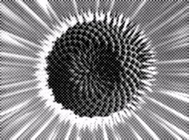
Figure 11: Close-up of a daisy floret
With the naked eye, we can easily see the “spirals” that form outward from the center. These are called “parastiches”, and surprisingly, there is a different number arranged clockwise compared to counter-clockwise. In the daisy above, there are 34 clockwise spirals and 21 counter-clockwise. Domestic sunflowers have 34 and 55 parastiches, respectively, and the pattern can also be seen in pine cones, fir cones, and pineapples, too. [Prusinkiewicz, 1990, pp. 102-106]
Hofstadter's AI Assignment
Douglas Hofstadter defined sequences similar to the Fibonacci sequence to be “triangular numbers” [Hofstadter, p. 14]. Each term in a triangular number is defined by summing a series of numbers according to a specific rule. For example, the fifth triangular number 15 is made up of adding (1+2+3+4+5):
1 3 6 10 15 21 28 36
45 55 66 78 91 ...
For his system, there are also “square numbers”, “pentagonal numbers”, “hexagonal numbers”, and so on. He notes that most people would be surprised to realize that the series of squares (“1, 4, 9, 16, 25, 36, 49, …”) can be created by summing the first n odd numbers. For example, the fifth square is 25, which is also 1 + 3 + 5 + 7 + 9.
For the class he was teaching on artificial intelligence, Hofstadter asked his students to write a computer program that would use a library filled with sequences such as the triangular numbers above, the series of prime numbers, of even a simple linear ordering such as “1 2 3 4 5…” or “2 4 6 8 10…”.
Hofstadter realized that the assignment would quickly turn into a searching algorithm such as depth-first search or breadth-first search (similar to many real-world artificial intelligence problems). The students would take the given sequence of numbers and transform it with one of the templates in the library. A metric would tell the students how close or far away they were from the target sequence, and if needed, several more transformations would be applied. This is similar to the way Prolog searches and backtracks through its rule set to proof the truth (or falsehood) of various axioms.
At the end of the semester, Hofstadter had a competition, and the best student entries were given new numerical sequences to solve. Surprisingly, several of the programs worked extremely well, even when given new domains of sequences that they had never seen. Hofstadter talks about how the assignment led into a class discussion of chess-playing computers and music synthesis.
Guessing and Overfitting
Finally, Hofstadter wishes that he would have structured his assignment so that the students were only given part of the sequence, and they would have to solve it or ask for another number. This way, they couldn't write an algorithm that only generated the test data but couldn't extrapolate the next number in the sequence.
In numerical analysis, we can create an n-degree polynomial that will fit (n-1) points of data. For example n = 2 points create a straight line, while n = 3 creates a parabola. This new line-fit can be used to interpolate unknown values that were not given. However, this method is extremely bad for extrapolating new values. For example, if the old data point were in the range [a,b], the interpolating function can have extremely large error for f(x) < a or f(x) > b.
The field of connectionism and neural networks displays this problem by the phenomena of “overfitting”. If we train and test on the same set of data, there is a danger that the final functions will match the data exactly, causing huge errors with data that isn't in the training set.
If we are trying to “explain” a series of numbers (or if we try to guess the next number in a series), we could think of this as writing a computer program that would generate that series. For example, you could envision a rule that says, “The sequence is the numbers 50, 55, 62, 71, 79, followed by the square root of negative one”. Written as a computer program, this sequence is valid even if the rule seems arbitrary. In fact, any answer, be it “-1”, “1,024”, or “pi” could be possibly rationalized as correct, given an arcane enough explanation.
Often, the “correct” answer to a simplest and most elegant answer is the one that can be written down quickly. Algorithmic complexity can be a good measure for how “random” a number sequence is.
Algorithmic Complexity
In this definition, the digits in the number pi are not random, because there exist several algorithms that calculate it completely. In fact, this corresponds to human intuition: people who can memorize numbers easily often comment that how “hard” of easy it is to remember a sequence depends on how easy they can store a mnemonic method in their brain that may have little to do with the statistical properties of the number. [xv]
For example, take a string discovered by David G. Champernowne. It is the set of all possible one-digit combinations (there are two: 0 and 1), then the set of all two-digits combination (out of four possible), and so on:
0,1,00,01,10,11,000,001,010,011,100,101,110,111,0000,etc.
It can be shown that this string is random (“typical” in Shannon's terminology), because it includes as many zeros as ones, and that every two-digit sequence is also uniformly represented. This will possibly be a very small error caused by the fact that the string has a beginning and an end that can't be combined into a pattern, but that can be solved by reversing the series into a mirror or itself:
etc.,000,11,10,01,00,1,0,0,1,00,01,10,11,000,etc.
However, this string is not random at all to a human eye. In fact, it can be written in a C program using recursion in only four lines of code! Better yet, we can create a function written in numbers, that when translated, produces a second sequence.
To state it more precisely, the complexity of the algorithm depends on the complexity of a Universal Turing Machine needed to fully describe the sequence. However, we run into two problems here. First of all, there is no penalty if the Turing machine implements simple rules, but takes infinite time to calculate the sequence (like a calculation of pi). Also, there are several different types of Turing machines, and what may be difficult for one machine to calculate may be easy for another, or vice-versa. In that case, which one “wins”? How complex is the original sequence?
Chaitin's Approach to Complexity
One problem with algorithmic complexity is that it is hard to perform operations using those complexity measures. If two strings are completely independent, the complexity of the concatenated string is sum of the two. In other words, you have to give an algorithm on how to produce the first string, and then start over for the second string. If there is a lot of shared information between the two strings, you might be able to write one program to describe them both (such as a string and its exact inverse).
Gregory Chaitin gives another idea of complexity in his paper, “Complexity and Randomness in Mathematics”, given as a talk for the 1991 “Problems in Complexity” symposium in Barcelona Spain [Chaitin, pp. 191-195]. Suppose you wanted transmit the string “101” and “000. Well, if you knew beforehand that the strings were of equal length, you could transmit the concatenated string “101000”. However, if the second one is longer (such as “00000”), that trick won't work. Chaitin suggests doubling each string and adding an “01” marker at the end to show where the delineation occurs.
<101,00000>
→ <11 00 11 01 00 00 00 00 00 01>


1  0  1     0  0  0  0  0
So, now the complexity is bounded by twice the sum of their individual entropy:
![]()
However, we could also add a “header” that defines how many bits are in each message. To help decoding the string, the header will consist of doubled digits (followed by that “01” stop code), and then the original string:
<11
11 01 101 11 00 11 01 00000>


1  1         1  0  1
The “11” corresponds to the number “3”, which is the length of the string found after the stop code. Likewise, “101” relates to the five digit sequence of the next string. Now our concatenated complexity is:
![]()
Chaitin goes further to put
a second header in front of the first header!

<11
00 01 11 101 11 11 01 101 00000>

 [1
0   ] 3     [1  1  ]  5
…and the length is:
![]()
This is a bit confusing, but the first code “10” tells the decoder that the next two-digit string is going to specify the length of the “real” string. When the decoder find the length “3”, we read in three more digits and we're done for the first part. Even though this scheme seems a lot more complex, we have only increased the length of the final string from 22 digits to 25. Now the total length is:
![]()
With headers of headers of headers, our length turns into:
![]()
And so on. Now, me have a complexity measure that can be calculated given two separate strings. Instead of a simple entropy n, we can recursively find a limit to the entropy n plus the complexity of n. This measure has a lot of advantages, but is still being developed. Chaitin admits, “The development of this new information theory was not as dramatically abrupt as was the case with Shannon's versions. It was not until the 1970s that I corrected the initial definitions” [Chaitin, p. 206]. There might still be a lot of work to be done.
A Gardner Puzzle
Martin Gardner has a great puzzle in his book “Knotted Doughnuts and Other Mathematical Entertainments”. Try to figure out the principle that orders the following digits from 0 to 9:
8 5 4 9 1 7 6 3 2 0
When the answer was printed in the Massachusetts Institute of Technology's “Technology Review”, a reader named Benson P. Ho sent in an alternate answer. In his solution, he drew a “V” of numbers that added up to a sum. First, subtract the number to the right of each “V” from the digit on the left. If the result is negative, add 10. So, 7-6=1 and 4-9(+10)=5. Then, the pairs of arrows point to the sum of the two digits, where if the sum is greater than 10, just subtract 10.
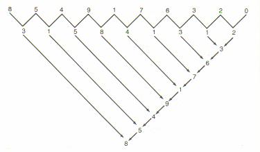
Figure 12: Benson P. Ho's Solution
Notice how the same series of numbers appears going up the right side of arrows. The probability of any two series appears by random chance is one part in 10 trillion or 0.000000000001%. The “correct” solution given by the Technology Review seems mundane in comparison: the numbers are in alphabetic order when spelled out as: “eight”, “five”, “four”, “nine”, “one”, “seven”, “six”, “three”, “two”, and “zero”. There appears to be is a seemingly huge amount of information stored in Ho's solution. Either it is an amazing co-incidence that the series would have a “V” property like Ho suggests, or perhaps there is something unique and strange about the alphabetic ordering of those numbers.
As it turns out, neither answer is the case. There is nothing interesting about Ho's method. In fact, any ten-digit string of numbers would produce the same results. So, this example might contradict an algorithmic interpretation of complexity. We could define an algorithm to a computer based on alphabetic sorting, but we would need a lot of auxiliary information first. We would need to match each number with its alphabetic spelling, and then define an ordering that is much larger than simply specifying an arbitrary ordering of the ten numbers. Ho's solution forms an algorithm that is shorter, but is evidently content- and information-free.
Or, what if there exists an algorithm to specify complex irrational number but we don't know what it is? Is the complexity of a series dependent on how clever we can be at writing algorithms? If that is the case, we could say that all series have the same complexity to a bad mathematician. To say that a simpler algorithm exists doesn't give us any clues on how to find that algorithm, and so the measure is may not be very helpful. Perhaps we will come up with a better idea of complexity in the future. It would be a lot easier than trying to figure out a way to write better algorithms!