Return to the home page for Patrick Kellogg
For this project, I wanted to model the efferent auditory system in human beings. So, I created a neural network that could recognize different types of sound. Then, I trained the network on four WAV files that had been pre-processed by a Fourier transform into a "spectragram". Finally, I found an "optimal input" for each sound class and used this to simulate the attenuation caused by efferent signals. Together, I think that the three steps create a vivid and useful model of human hearing.
I was inspired to do this project last year, when I realized that the same topics discussed in Prof. Howard Wachtel's "Neural Signals" class were quite similar to algorithms I was studying in my computer science classes. Overall, this project was fun to do and I am grateful I was given the forum to do it. The results are very interesting, although not very conclusive, due to the shaky (and almost "black art") nature of neural networks. Perhaps I can continue this work in the future, especially if I can find some clinical data to compare to my statistical model.
Most people aren't surprised that there are electrical impulses that travel from the ear to the brain. After all, that's the definition of hearing. However, there are also neural signals that travel back from the brain to the ear. The first type of signals is called "afferent", while the second is called "efferent".
A good example an afferent signal (toward the brain) is the sense of touch. Whenever you feel heat or pain, an electrical stimulus follows a path up the spinal cord to be processed by the brain. Efferent signals (away from the brain), on the other hand, exist where the brain wants to perform an action, like activating muscles that pull your hand back from heat or fire. Complicated actions, such as riding a bicycle or throwing a ball, can only be accomplished by combination of afferent and efferent signals.
What efferent hearing actually does is control how much sound the brain hears. Human beings can never completely stop hearing since we can't close our ears. However, we can do the next best thing— we can attenuate (that is, decrease) the level of some frequencies that reach the brain. All of this is done subconsciously, and due to some "balancing" mechanism in the brain, we are never aware of it happening.
As an example of this phenomenon, imagine you are at a party full of men talking loudly. If you were searching for a female friend amid the crowd, you could unconsciously "shut off" you lower frequency range to concentrate on the upper frequencies where her voice would be heard. Animals probably evolved this talent so they could hear prey approaching, or they could be wary of unusual sounds among ambient noise. It might also explain why it's often hard to get someone's attention if you talk to them while they are watching television.
The entire structure of the ear, from the fleshy outer ear to the odd "hammer-and-anvil" on the inner ear, all serve as a preliminary signal processing step for incoming sound. The outer ears channels the sound and directs it (and may also perform some complex binaural direction that we don't understand yet [Hawkins 15-27]) while the inner ear is a clumsy but effective amplifier that demonstrate some non-linear filtering.
Eventually, the sound reaches the cochlea, which looks like a small coil. If stretched out, the cochlea would be a tube divided lengthwise into two parts by the "basilar membrane". Sound waves are reflected through one side of the basilar membrane, off the "scala tympani" at the end of the tube, and back down the other side. All of this acts like a real-time Fourier transform that turns sound into its frequency components.
Along the basilar membrane are little sensing mechanisms called "hair cells". Although not related to real hair, they stick out like bristles and must have looked strange when viewed under early microscopes. When the hair cells vibrate, they send an electrical signal to the auditory nerve, which sums them up and carries the signal to the brain. Hair cells close to the scala tympani (or, in other words, the end of the cochlear tube) respond to high frequencies, while hair cells farther away respond to low frequencies.
Hair cells can be damaged by too much stimulation, and they lose their range of motion as they age, resulting in hearing loss in older people. Efferent signals take advantage of the fact that by tightening the muscle surrounding a section of hair cells, those hair cells can no longer move freely and are held rigid. By freezing different ranges of hair cells, the cochlea can act as a low-pass, high-pass, or band-pass filter. Plus, all of the filtering is done in "real time" with complex interactions that any acoustical engineer would be hard-pressed to duplicate.
Over the last thirty years or so, computer scientists have developed a new tool for creating statistical models: the "neural network". Contrary to its name, neural networks aren't used merely to model biological or electrical phenomenon, but have been used to analyze stock market data, weather, fluid mechanics, even racehorse results and backgammon. All in all, neural networks are just another statistical tool, albeit a very interesting and versatile one.
The base unit of a neural network is a neuron or "unit". Simply put, a unit adds up its input values and outputs one sum. Then, that output act as one of many inputs for another unit. That's all, nothing tricky or human-like yet. The fascinating twist to neural networks is that the error value of how far away an output value is from a desired value is also a kind of signal. The error can be "backpropagated" backwards through the neural network, changing the "weights" of all the outputs. This interesting discovery allows neural networks to "learn" how to turn on a given output neuron if given a pattern of inputs. The process of learning by changing the weights of units is called "gradient descent".
The mathematics of gradient descent proves that a neural network can learn any given input if given a small enough "learning rate" and enough time. Unfortunately, the amount of time needed could theoretically be infinite. So, we are often happy with a "close enough" network whose error rate that falls below a desired value.
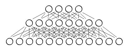
My neural network contains 20 units in the input layer, 10 in the hidden layer, and as many units in the output layer as there are sounds. So, if only sound #2 is present out of four of them, ideally I'd like the output layer to be -1/+1/-1/-1. Nothing can really be said about the middle layer, and trying to gain information from looking at middle layer values is almost always pointless. The input layer, on the other hand, has 20 units because I have divided each input sound into 20 frequency "bins".
All sound is fundamentally made up of sine waves of varying frequencies and amplitudes. The "Fourier transform" is a mathematical algorithm to decompose a sound into its spectrum. Since the Fourier transform likes its input to be a power of 2 (like 26=64), I sampled my sounds at 10240 Hz, a little better than the quality of a telephone conversation. Actually I'm fudging a little here— the sound was sampled at 11025 Hz, but I am pretending it is a slower frequency throughout. As long as I am consistent (and not trying to recognize sounds in "real time", I think I'm all right. I'm also leaving out such details as normalization, "Hamming windows", and "critical band theory".
The sound is turned into an array of 20 rows by 30 columns. Each row represents a frequency range, with the first row those sine components from 180 to 300 Hz, all the way up to the last one encompassing columns representing 4000 to 4500 Hz. Note that the maximum possible frequency bin is half of the sampling rate due to the Nyquist Sampling Theorem. Each column represents the frequencies present during a 0.1 second window of sampling. The "windowing" of discrete time sampling often causes problems, but is a limitation that I had to accept. After all pre-processing steps are done, the user is left with a pretty "spectragram", where they can see the frequency components fade in and out of strength.
For my test, I sampled four sounds that were readily available in my computer room: an air conditioning fan, a television set tuned to static, the radio playing, and the sound of window blinds opening and closing. As it turned out, the blinds and the television were the hardest for the neural net to discriminate, possibly because they both have a very "white noise" sound that is made up of many frequencies.
Once all four sounds were prepared as spectragrams, they were saved into a MATLAB-readable file. My neural network code had a routine to choose a sound randomly and train the weights using backpropagation and gradient descent. I didn't use an "early stopping" technique, but instead waited until the total sum error was under a certain value (which usually occurred after 200 or 300 training iterations). I also compared the network's performance to four "testing" sounds that I had prepared into spectragrams, but which came from a different sample. This prevented "overfitting" or the annoying habit of a neural network to memorize the input sounds but to reject any sound that isn't exactly the same.
With the neural network trained, I proceeded to find an input pattern that gave the strongest desired output. This type of procedure is often called "Bayesian" or "post-conditional" analysis. My advisor, Michael Mozer, suggested that I could use gradient descent again to find dE/dI, that is, the change in error with respect to the input. His method worked quite well, although there were a lot of "local minima" that I did not test for. In other words, there are many patterns of frequencies that the neural network might recognize as an air conditioner, and I'm not sure that I found the optimal one over all patterns.
Gradually, my neural network found an "optimal input" for each sound class. Often, it was nice to see that each optimal input was almost orthogonal (that is, it though a certain band of frequencies was important for a given sound but was unimportant for all others). However, sometimes when the code ran, the optimal inputs overlapped, especially between the white-noise sounds. I attribute this to the problems with local minima, and to the fact that neural networks are very sensitive to the initial random values of the net. Sometimes, it seems, I started with a "good" set of variables.
I consider the optimal inputs for each sound to be what the brain would use to create an efferent signal. Since the optimal input was already normalized to a 0-to-1 range, I could simply multiply it with an incoming pattern before passing the input through the neural network. If I wanted to recognize sound #2, I would use the optimal pattern #2 as a sort of attenuating filter for all inputs.
As it turned out, this method often created good results. I applied each attenuating filter in turn and examined how well the neural network recognized the original sound. In the graph below, the red/teal/yellow/red bars signify the filters for the optimal sounds 1/2/3/4 respectively. In the first group, applying the #1 filter allowed the net to recognize sound #1 easier that with any other filter. The same pattern worked for the other sounds (red filter #4 was the best for sound #4, yellow #3 filter for sound #3). The only discrepancy was sound number two, which did best with filter #2, but also performed quite well with its own filter.
Actually, I ran the simulation a number of times, with similar results. Often each sound would "match up" with is own filter. However, often a sound would do better (or just about as well) with another filter. As a result, I don't think my results are very impressive or conclusive. However, it's a good start, and I 'd like to attempt the same test with different sounds, a group of ten or more sounds, or perhaps a different architecture to my neural network (like a different number of units in the "hidden" layer).
There were many limitations that I had to accept for this project, just like any other scientific model. The idea was to simplify the phenomenon, and in doing so, hopefully none of the important details were lost.
This project was a lot of fun to do, although I don't think I have proven anything. The results were not as dramatic or conclusive as I had hoped. I was fun, though, to see how gradient descent "found" the optimal values for both the network weights and the optimal input. The same code (with a small modification) performed identical tasks.
I would like to find some clinical data to compare to my results. Also, human hearing is a give-and-take process where the brain learns while it sends new efferent signals. My model, on the other hand, learns first and then models efferent hearing without modifying the weights. A real-time simulation would be a lot of fun to see, although I think my neural network code would have to be moved into hardware for it to work properly.
This project gave me some insight to the cognitive psychology theory of attention. There are many books written on this topic, most from a high-level philosophical level. However, I think that attention is merely a mathematical construct. For example, it my project, simply using a filter related to a given sound class changed how all future sounds were interpreted, whether they belonged to that class or not. Even better, the methods used to generate the filters were the same as the ones that trained the network. This leads me to believe that something similar actually occurs in the human brain whenever we try to "listen for" or recognize a sound we have heard before.
For my upcoming Master's thesis, I would like to concentrate on sound production as well as sound recognition. They are like two sides of the same coin. Theoretically, if you can extract the salient features that make a sound distinctive, you could reproduce and modify similar sounds. I would like to study such cutting-edge tools as Independent Component Analysis (ICA), fractal compression of sound, and wavelet decomposition. Perhaps these tools can remove some of the limitations of my project and I will return to the idea of modeling efferent hearing again someday.
Bengio, Yoshua Neural Networks for Speech and Sequence Recognition International Thomson Computer Press 1996
Hawkins, Harold L., Teresa A. McMullen, Arthur N. Popper, and Richard R. Fay (editors) "Auditory Computation" Springer 1996
Moore, Brian C.J., Roy D. Patterson (editors) "Auditory Frequency Selectivity" NATO ASI Series, Series A: Life Sciences Vol. 119 Plenum Press 1986
Owens, F.J. "Signal Processing of Speech" McGraw-Hill 1993
Press, William H. et. al. "Numerical Recipes in C" Second Edition Cambridge University Press, 1996
Rosen, Stuart, and Peter Howell "Signals and Systems for Speech and Hearing" Academic Press (Harcourt Brace Jovanovich) 1991
Sahey, Tony L., Richard H. Nodar, and Frank E. Musiek "Efferent Auditory System" Singular Publishing Group, Inc. 1997